Intro

Let's discuss the perceptron and a trick that can be used to simplify (a bit) an analysis of many supervised ML algorithms.

So what is perceptron?

It's probably the simplest binary classification algorithm. It tries to find a decision boundary that can be modeled as a $D-1$-dimensional plane where $D$ is the number of features in input data. So we are basically cutting our space into two pieces. The class of a sample is then decided based on the part of the space to which the sample falls.

A 2D example is in the following picture:

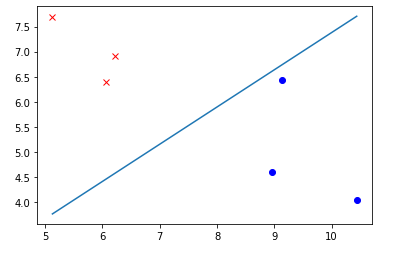
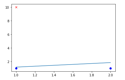
Notice how close is one of the blue points to the boundary. This is characteristic property of perceptron. It is not in any way optimizing where the boundary is placed. All it does is dividing the plane so that training examples are properly classified. Because of that, you can get very screwed boundaries like the following:

Also it won't work for data that aren't linearly separable:

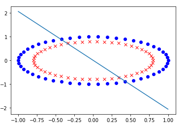
It looks pretty useless, right? And yes, it's pretty weak but it's also super simple. All you need to have for this algorithm is a vector of weights $\textbf{w}$ and scaler-variable $b$ called bias. Let's define the possible classes for our data as $\{1, -1\}$. Then we can define prediction for $\textbf{x}_i$ as follows $$y_i = \text{sign}(\textbf{x}_i^T \textbf{w} + b).$$

Observe that whenever $y_i$ is incorrect the following holds $t_i y_i < 0$. This is a good moment to pause and see that the inequality really works.

With it in our toolbox we can define loss as $$L = \max(0, - t_i y_i) = \max(0, - t_i (\textbf{x}_i^T \textbf{w} + b)).$$ This we need to minimize across all training examples. It's nice to notice that the loss can be also written as $$L = \text{ReLU}(- t_i y_i),$$ The training isn't much harder as we'll see in a second. But prior to it let's discuss hiding the bias.

Hiding bias

Hiding bias is a neat trick that will simplify both analysis and the update rule. We are going to hide the bias in $\textbf{w}$ so that we will only need to derive update rules for this one vector. Note that this method can be used with many other ML algorithms too.

Let's rewrite the dot product in prediction as $$\textbf{x}_i^T \textbf{w} + b = x_1 w_1 + x_2 w_2 + \dots + x_D w_D +b = x_1 w_1 + x_2 w_2 + \dots + x_D w_D + 1 b.$$

How is this useful? Observe the last term $1 b$. There is a multiplication of two scalars like in the preceding terms. This allows us to rewrite the whole thing as yet another dot product $$(x_1, x_2, \dots, x_D, 1) \cdot (w_1, w_2, \dots, w_D, b).$$

Suddenly $b$ disappeared and we are dealing with new weights and $x$ vectors with dimensionality $D+1$. Prediction is now defined as $$y_i = \text{sign}(\textbf{x}_i^T \textbf{w})$$ and similarly for the loss.

Putting it all together

With bias hidden there is no need to think much about updating it. We want to minimize $$\max(0, - t_i \textbf{x}_i^T \textbf{w})$$ with a bit of calculus, we arrive at the following update rule $$\textbf{w} \leftarrow \textbf{w} + t_i \textbf{x}_i$$ which is used whenever the example is classified incorrectly. For correctly classified examples we do nothing.

It's good to note that using derivatives to get the update rule is a bit overkill. I recommend you to try this on paper (it should give better intuition than my explanation). Imagine what's happening. We have two vectors $\textbf{w}, \textbf{x}_i$ and in prediction we are basicaly calculating their cosine similarity. The result is positive for an angle between vectors which is less than $90^\circ$ and negative for more than $90^\circ$. Now when there is an incorrectly classified example the angle between $\textbf{w}, \textbf{x}_i$ is either too small or too great. By adding $t_i \textbf{x}_i$ to the weights vector we are rotating it in a direction that is favorable to us. For $t_i = 1$ the angle is getting smaller, for $t_i = -1$ the vectors are drifting more appart.

Sidenotes

If you're interested in the code that was used to generate pictures in this article, you can look here.

If you found a mistake or want to share some thoughts on perceptron, you can write to me here.

If you are looking for more on perceptron, you may enjoy the following

• Slides from my ML teacher. They are well prepared and use pretty much the same notation as this article.
• To get a more intuition on linear-separable data and biological inspiration behind the perceptron look here.